
Everything in the Demo tier, plus the layers a real decision needs
Building and solving on the Demo tier costs nothing. The paid tier adds the tools for the work around the solve: comparing futures, phasing the build, and keeping every result at full detail.
Build, solve and export unlimited models
No ceiling on the size of the model. The paid tier lifts the Demo tier's caps on components, snapshots, solves per day and solve time, so a whole state's generation fleet, a multi-year investment pathway or a plant with hundreds of process steps solves as one network.
Every model you build leaves with you: download it as a project file or as an open PyPSA netCDF, and bring your own netCDF networks in the same way.
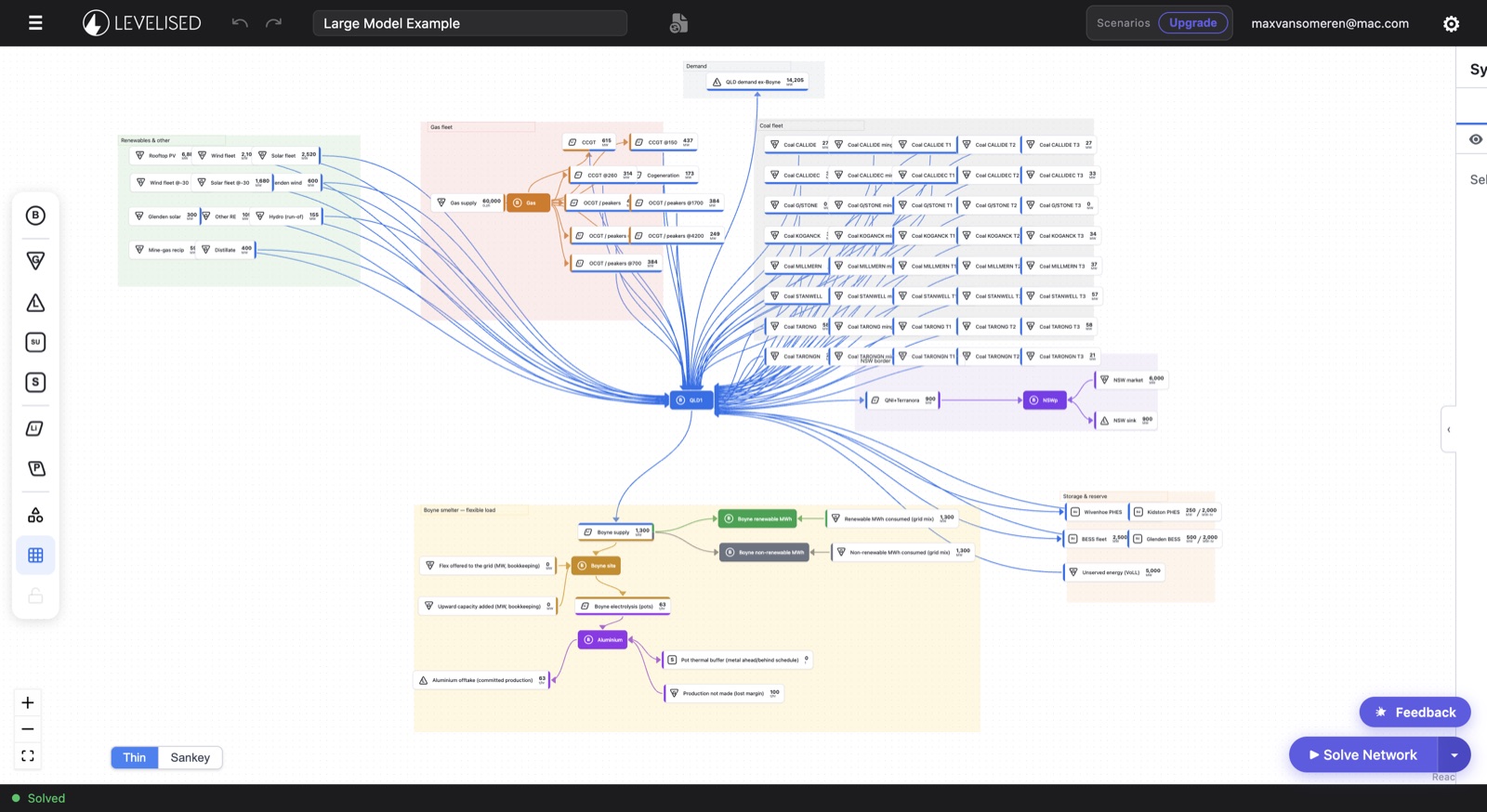
Scenario management
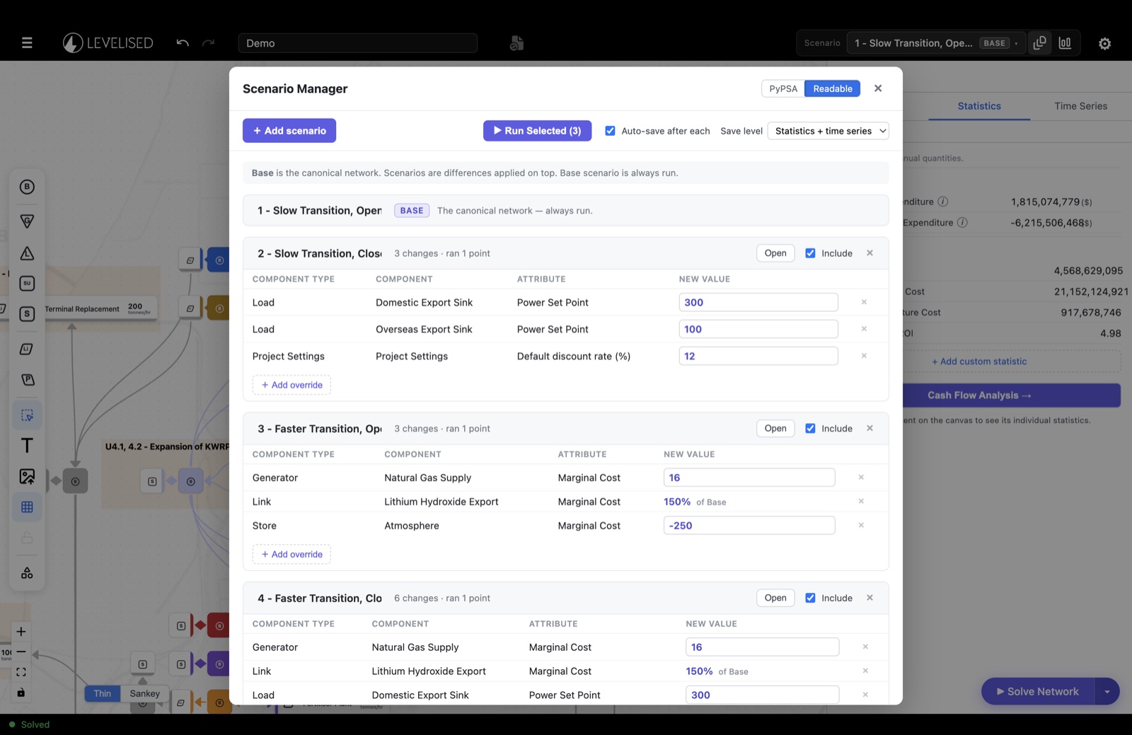
Compare how your results change across different futures. A scenario is a set of differences applied on top of your base network (change the cost, efficiency or scale of any component), so one model carries every case you need to argue.
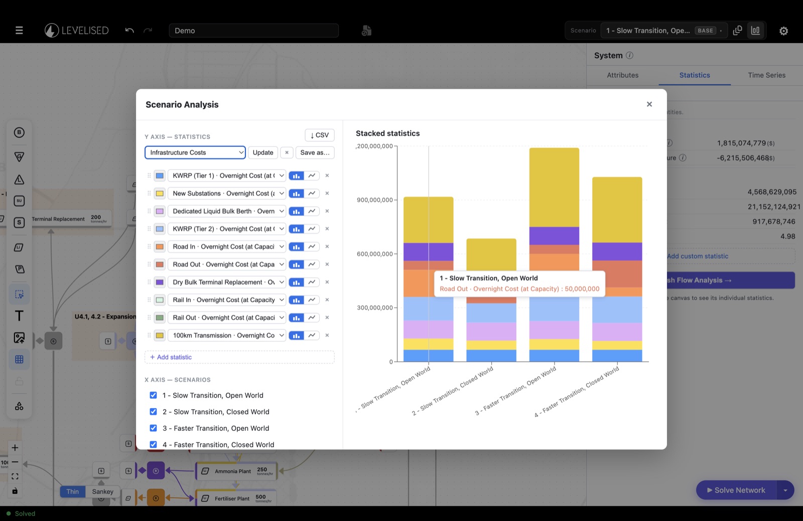
Run one scenario or all of them in a batch, then put them side by side in the scenario analysis toolbox: any statistic, stacked across scenarios, exportable to CSV.
Multi-period analysis
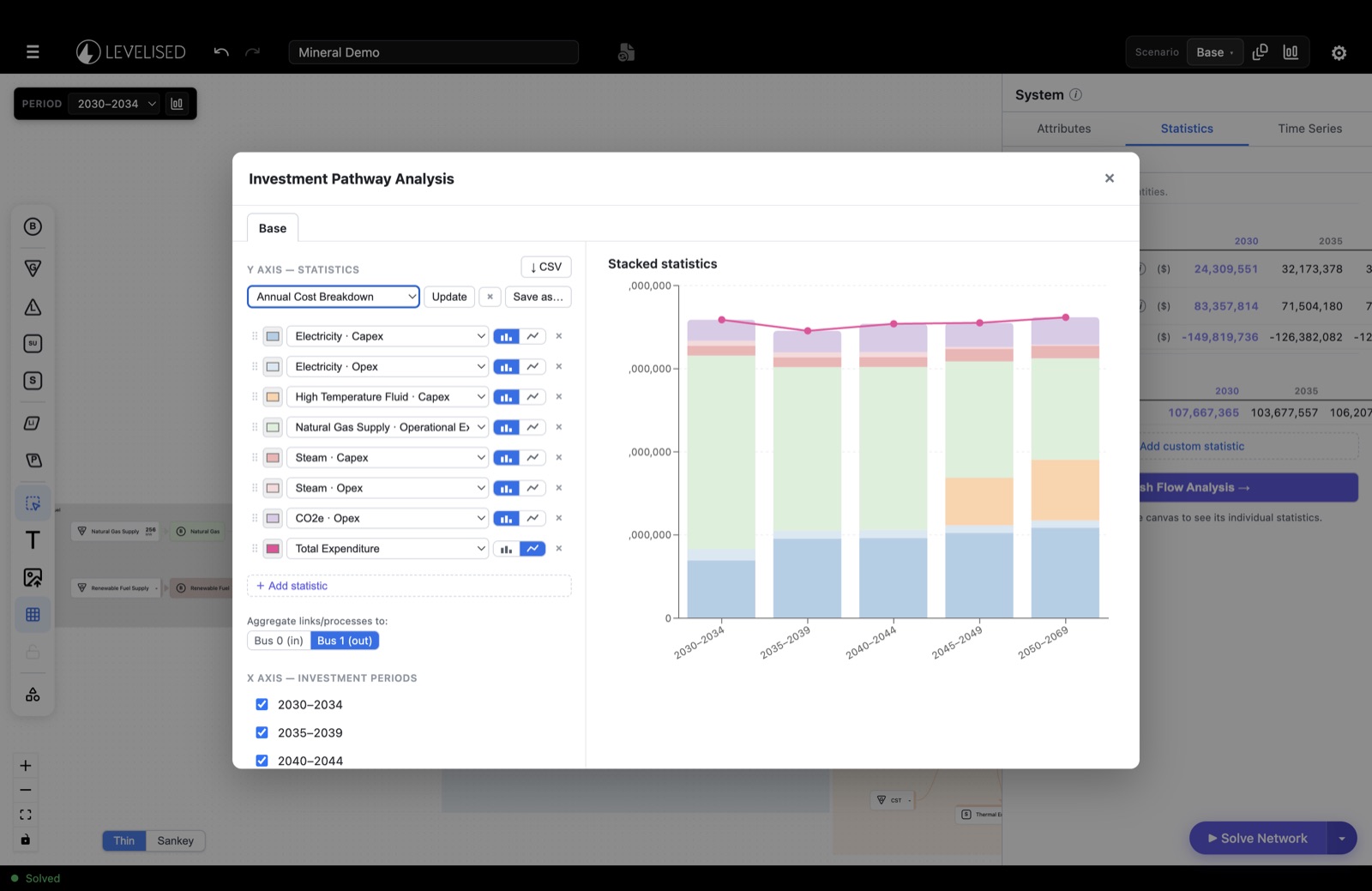
If your project proceeds in phases, multi-period analysis is for you. Split the horizon into investment periods, set different objectives and constraints for each (an emissions cap that tightens, a load that grows, a contract that expires), and the optimiser builds the least-cost investment pathway across the whole life cycle, not one year at a time.
The pathway analysis view shows what gets built when, and what each period's decisions cost.
Custom optimisation constraints and objectives
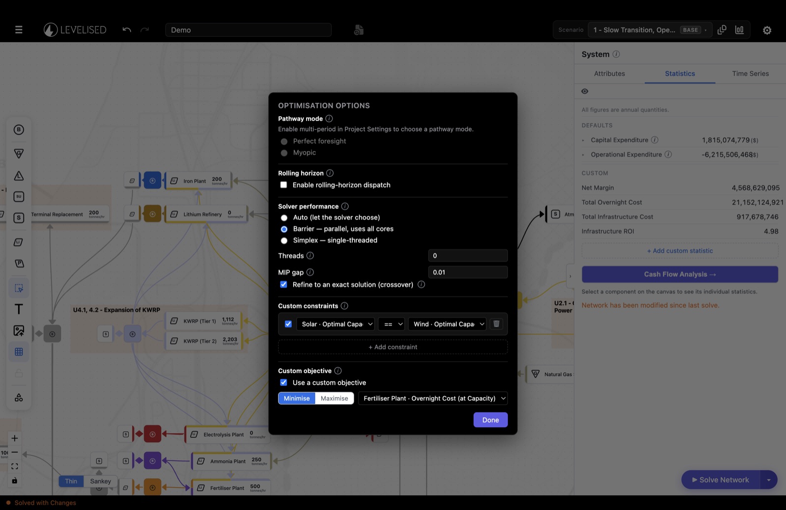
Need more control over the optimisation? Add your own constraints: a fixed ratio between solar and wind capacity, a floor on firm supply, a limit the default formulation doesn't know about. They become part of the solve, not a manual check afterwards.
You can also swap the objective itself: minimise or maximise any statistic in the model, not just total system cost. Solver performance options (algorithm, threads, MIP gap) come with it.
Full time-series results in the cloud
On the Demo tier, cloud saves keep your model and its results at statistics level: totals, costs and key metrics for every component. The paid tier saves the full-size file, every hourly time series included, so a solved model reopens exactly as you left it.
That means dispatch profiles, storage state of charge and hourly prices are all there when you come back, ready for the charts and the exports, with no need to re-run the solve.
And more
Something you need that isn't here? Tell us. Your answer shapes what we build next.